So, long time, no post. However these last couple weeks have been crucial for my thesis and all the extras and the next week is not going to be fun either since I hand in everything on Tuesday. *sarcastic yay!*
However, I did say I would put up my poster. Enjoy. Let me know how cool you think it is on a scale from -10 to 10. :-)
Soon I will link this to the website I am producing for the project so you have the complete picture of my year's work.
Showing posts with label chaos theory. Show all posts
Showing posts with label chaos theory. Show all posts
Wednesday, 27 April 2011

Friday, 8 April 2011
On a less serious note
So, I realised just a few minutes ago that I haven't written about chaotic attractors in all their splendour. An incredible oversight on my part. These objects are achingly beautiful and intricately complex in form. They arise in phase space (I believe I have covered this) in certain parameter regions of systems. Their fractal geometry means that dynamics is incredibly sensitive on them and while trajectories will follow the path of the attractor (duh! attracting :-) ), there is no predicting which exact part of the attractor it will land on and follow round or ultimately where it will end up. The attractor is fixed, the trajectories are not. A nice succinct explanation is available here.
The one that ties in closest to my work is the Lorenz attractor. The three dimensional system for describing turbulence gives birth to an amazing structure. This attractor is where the 'butterfly effect' expression originated. The attractor itself is geometrically between two and three dimensions and winds itself around two points.
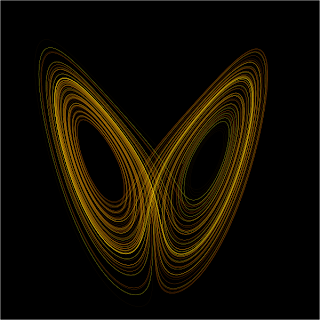
The image (from wiki) shows exactly this. Where the trajectories 'cross' in this two-dimensional visualisation is actually where they layer over each other - manifolds cannot intersect (the unstable manifold exactly describes the attractor). The view is better in 3d. The fractal (Hausdorff) dimension of the attractor is about 2.06.
Other systems with strange attractors are the Rossler system and Henon map. This page gives a nice description and a few images.
As a side note: for those of you who read and enjoyed 'Harry Potter and the Methods of Rationality' or 'Luminosity' I would recommend this strangely named (but you'll understand all too soon) 'Baby Eating Aliens' also from the Less Wrong family and the (there is a theme here, no?) 'Harry Potter and the Wastelands of Time' if you like a bit of complex, epic writing with lots of action and magic!
Enjoy! Also, something to look forward to: I hope to have my poster available for you lot next time I post. :D
Doh! Almost forgot. One of the lecturers at my university (Hinke Osinga) actually crocheted the Lorenz stable manifold! If you want to know how, read this!
Incidentally, my project supervisor is the Bernd Krauskopf mentioned in the article. And yes, it is one of their Christmas decorations. ;)
The one that ties in closest to my work is the Lorenz attractor. The three dimensional system for describing turbulence gives birth to an amazing structure. This attractor is where the 'butterfly effect' expression originated. The attractor itself is geometrically between two and three dimensions and winds itself around two points.

The image (from wiki) shows exactly this. Where the trajectories 'cross' in this two-dimensional visualisation is actually where they layer over each other - manifolds cannot intersect (the unstable manifold exactly describes the attractor). The view is better in 3d. The fractal (Hausdorff) dimension of the attractor is about 2.06.
Other systems with strange attractors are the Rossler system and Henon map. This page gives a nice description and a few images.
As a side note: for those of you who read and enjoyed 'Harry Potter and the Methods of Rationality' or 'Luminosity' I would recommend this strangely named (but you'll understand all too soon) 'Baby Eating Aliens' also from the Less Wrong family and the (there is a theme here, no?) 'Harry Potter and the Wastelands of Time' if you like a bit of complex, epic writing with lots of action and magic!
Enjoy! Also, something to look forward to: I hope to have my poster available for you lot next time I post. :D
Doh! Almost forgot. One of the lecturers at my university (Hinke Osinga) actually crocheted the Lorenz stable manifold! If you want to know how, read this!
Incidentally, my project supervisor is the Bernd Krauskopf mentioned in the article. And yes, it is one of their Christmas decorations. ;)
Wednesday, 30 March 2011
Horseshoe Chaos
While I struggle with supposedly impossible inversions, I'd like to introduce you all to Smale's horseshoe. This object is where the definition of chaos originates yet it is a relatively simple idea.
You start with a square. Squish is down and pull it out to the sides then bend it at the halfway point so it looks like a horseshoe. Then replace it over the square so that the two lengths form vertical strips on the square. This is the basic transformation of the horseshoe map. It is also invertible. Take the bent strips, rotate back to horizontal, and unbend it then squish it in from the sides and pull from the top and bottom then you get the square again. If you do this inversion again you get strips intersection horizontally.
Repeatedly performing the forward transformations you get more and increasingly thin vertical strips: 2 strips become 4, 4 strips become 8 i.e. each strip gets two thinner strips within it at each iteration. Doing the same backwards, you get lots of increasingly thinner horizontal strips. The points in the strips are the points that remain in the set at that iteration. Most points leave after even just a few iterations in either direction.
If you overlay the two directions, the points at the intersections that remain in the square under all iterations (if you iterate infinitely in either direction). This is the invariant set. This set is a Cantor set (disconnected and unstable fractal).
If you labelled each point with 0 or 1 at each iteration you could describe the positions of all the points in the square e.g. .0101 means a point that is in the 6th vertical strip after four iterations (the right hand strip of the left hand strip of the right hand strip of the left hand strip in the first iteration) or
 If you can see that...sorry if it's too small.
Since you can do this in both directions, the whole dynamics of any point in the square can be described by it's bi-infinite sequence of positions.
Knowing this we can construct any orbit we like and we know it will describe at least one point in the square.
So we can make a periodic point: ...010101.0101010... which alternates from the left to the right. Since we have infinite lengths in both direction, we can make (uncountably) infinitely many of these periodic points.
Or we can make a non-periodic point: ...010001101100000.1010100110111... by, for example, 'counting' in binary as above or just by adding the wrong value to a periodic point i.e. ...01010101.0101011...is non-periodic. There are (uncountably) infinite of these too.
Among this set of non-periodic orbits we can find at least one that comes arbitrarily close to the invariant set. This is trivial since you can take just part of the sequence that describes a point in the invariant set and it would come as close as you like!
I hope you are following since I have just demonstrated that Smale's horseshoe perfectly defines chaos.
Chaotic motion must consist of the following:
- infinitely many periodic orbits
- non-periodic orbits
- dense orbits - ones that come arbitrarily close to any point in the set.
There tends also to be the condition of sensitive dependence on initial conditions but this can be shown through the dense orbits - you can take two sequences that are the same for any arbitrary iterations and in the next they can end up in two different strips i.e. they may start very close but can end up very far apart.
Voila!
Strogatz does give a very basic introduction but for a more detailed approach read the first chapter of "Elements of Applied Bifurcation Theory" by Yuri Kuznetsov. Wiki also has its own explanation.
You start with a square. Squish is down and pull it out to the sides then bend it at the halfway point so it looks like a horseshoe. Then replace it over the square so that the two lengths form vertical strips on the square. This is the basic transformation of the horseshoe map. It is also invertible. Take the bent strips, rotate back to horizontal, and unbend it then squish it in from the sides and pull from the top and bottom then you get the square again. If you do this inversion again you get strips intersection horizontally.
Repeatedly performing the forward transformations you get more and increasingly thin vertical strips: 2 strips become 4, 4 strips become 8 i.e. each strip gets two thinner strips within it at each iteration. Doing the same backwards, you get lots of increasingly thinner horizontal strips. The points in the strips are the points that remain in the set at that iteration. Most points leave after even just a few iterations in either direction.
If you overlay the two directions, the points at the intersections that remain in the square under all iterations (if you iterate infinitely in either direction). This is the invariant set. This set is a Cantor set (disconnected and unstable fractal).
If you labelled each point with 0 or 1 at each iteration you could describe the positions of all the points in the square e.g. .0101 means a point that is in the 6th vertical strip after four iterations (the right hand strip of the left hand strip of the right hand strip of the left hand strip in the first iteration) or

Since you can do this in both directions, the whole dynamics of any point in the square can be described by it's bi-infinite sequence of positions.
Knowing this we can construct any orbit we like and we know it will describe at least one point in the square.
So we can make a periodic point: ...010101.0101010... which alternates from the left to the right. Since we have infinite lengths in both direction, we can make (uncountably) infinitely many of these periodic points.
Or we can make a non-periodic point: ...010001101100000.1010100110111... by, for example, 'counting' in binary as above or just by adding the wrong value to a periodic point i.e. ...01010101.0101011...is non-periodic. There are (uncountably) infinite of these too.
Among this set of non-periodic orbits we can find at least one that comes arbitrarily close to the invariant set. This is trivial since you can take just part of the sequence that describes a point in the invariant set and it would come as close as you like!
I hope you are following since I have just demonstrated that Smale's horseshoe perfectly defines chaos.
Chaotic motion must consist of the following:
- infinitely many periodic orbits
- non-periodic orbits
- dense orbits - ones that come arbitrarily close to any point in the set.
There tends also to be the condition of sensitive dependence on initial conditions but this can be shown through the dense orbits - you can take two sequences that are the same for any arbitrary iterations and in the next they can end up in two different strips i.e. they may start very close but can end up very far apart.
Voila!
Strogatz does give a very basic introduction but for a more detailed approach read the first chapter of "Elements of Applied Bifurcation Theory" by Yuri Kuznetsov. Wiki also has its own explanation.
Monday, 21 March 2011
How many drafts...?!
So here we are, nearing the end of my project. Well, actually there are six weeks left til I hand in my thesis but it doesn't feel like it. It feels more like two. :S
I've been asked to do two drafts already. A third one is coming up next week and I'll redo the current one into a fourth. After that they combine into a fifth. Then will follow a sixth from recommended improvements. I'll probably create another couple just for kicks! So that's at leasts one a week...a draft roughly for each month I've worked on it. I'm drowning in them!!
Ah well, at least it means I have shiny pictures for you this week. My draft task this week was to tell the story of one side of my research (decreasing lambda) as purely in images as possible. Obviously the details will be missing but I hope you enjoy the obvious progression and changes in images as lambda varies.
My image report draft is available here.
In other parts of my Masters world I am winding down on lectures and winding up for revision ready for exams in nine weeks. I want to try something new for my revision this year - sort of step it up a level. If anyone has any recommendations that would be very welcome. I have a few ideas but would like to augment these with other influences.
I also have to produce a poster and a website for my Masters project but I'll share them here first to get opinions! I will of course add a link to this blog in my website (cheeky I know!); maybe they'll give me extra marks for initiative and knowledge sharing never mind the pretty pictures!
I've been asked to do two drafts already. A third one is coming up next week and I'll redo the current one into a fourth. After that they combine into a fifth. Then will follow a sixth from recommended improvements. I'll probably create another couple just for kicks! So that's at leasts one a week...a draft roughly for each month I've worked on it. I'm drowning in them!!
Ah well, at least it means I have shiny pictures for you this week. My draft task this week was to tell the story of one side of my research (decreasing lambda) as purely in images as possible. Obviously the details will be missing but I hope you enjoy the obvious progression and changes in images as lambda varies.
My image report draft is available here.
In other parts of my Masters world I am winding down on lectures and winding up for revision ready for exams in nine weeks. I want to try something new for my revision this year - sort of step it up a level. If anyone has any recommendations that would be very welcome. I have a few ideas but would like to augment these with other influences.
I also have to produce a poster and a website for my Masters project but I'll share them here first to get opinions! I will of course add a link to this blog in my website (cheeky I know!); maybe they'll give me extra marks for initiative and knowledge sharing never mind the pretty pictures!
Tuesday, 15 March 2011
"To err is human"
And guess what?! I'm human. My error this time was such a small thing but it could have had huge consequences if I had not caught it when I had. Actually it would have been far better to have caught it much much earlier but I had no reason to see problems until this point.
I had successfully combined my manifold examination with the Julia Set calculations into one succinct image for each value of the parameter lambda. Nothing twigged until I sat there showing them to my supervisor and he commented that surely the attractors should actually lie within the prisoner set (the points that remained after the iteration). My manifolds also did not line up with the areas they would be expected to. This meant one of two things. Either I had some scaling issue (quite possible with all the jiggling around I had done to get them on the same image) or something was wrong with either side of the analysis (the MATLAB or DSTool code).
Since the DSTool code had been written by someone far more experienced in the area, it was to my code that I turned my attention to find the problem. Took me a while but (as the error rule says) when I found it it was easy to fix. I like to program quite efficiently and as I was testing the absolute value of Z at each iteration I had set
absZ = abs(Z)*abs(Z);
Now instead of square rooting this after I had tested it I had left it which meant that instead of just dividing by the square of abs(Z) at each iteration, it was dividing by the fourth power of abs(Z). Doh!
Thus all my Julia Set images were actually wrong. Re-running the (easily) corrected code showed just how wrong it had been. But it is fixed now and since then I have been working like stink to analyse the correct progression of Julia Sets.
One of the areas that I have now been progressing into was a direct result of the correction. Once the correct maps were generated, I added a further capability to zoom the section around the interesting circle region. This showed that the points within the Julia Set boundary were actually behaving very much like the stable set patterns seen by the PhD student I have been working with. So I have been expanding my analysis to include calculation of the stable set within the Julia Set boundary. This is likely to contribute to connectedness and other behaviours of the map I have already examined.
As far as I understand it, the stable set is the set of points that go to the attractor(s) via the stable manifold due to the existence of a saddle point. Some points, in the course of being iterated, will end up on the stable manifold or on the saddle itself before slowly reaching the attractor. The stable set is all the points back in time that forward in time end up at the stable manifold (thus more pre-image calculations are involved!).
I have calculated this for a few values and they show promising information - I would have inserted images here but the server is rejecting them...
They should help to determine what the hole actually does to the map at least in the limited sense that I am examining it.
Oh, also I would also have shown you the bifurcation progression through lambda but since the server is rejecting my images I won't be. I'll try next week. Sufficed to say that there is a lot going on. I'm not entirely sure I'll find it easy to stick to the 45 page limit. If anyone has any recommendations for that (things that they would find interesting so think should be included) please let me know. :-)
I had successfully combined my manifold examination with the Julia Set calculations into one succinct image for each value of the parameter lambda. Nothing twigged until I sat there showing them to my supervisor and he commented that surely the attractors should actually lie within the prisoner set (the points that remained after the iteration). My manifolds also did not line up with the areas they would be expected to. This meant one of two things. Either I had some scaling issue (quite possible with all the jiggling around I had done to get them on the same image) or something was wrong with either side of the analysis (the MATLAB or DSTool code).
Since the DSTool code had been written by someone far more experienced in the area, it was to my code that I turned my attention to find the problem. Took me a while but (as the error rule says) when I found it it was easy to fix. I like to program quite efficiently and as I was testing the absolute value of Z at each iteration I had set
absZ = abs(Z)*abs(Z);
Now instead of square rooting this after I had tested it I had left it which meant that instead of just dividing by the square of abs(Z) at each iteration, it was dividing by the fourth power of abs(Z). Doh!
Thus all my Julia Set images were actually wrong. Re-running the (easily) corrected code showed just how wrong it had been. But it is fixed now and since then I have been working like stink to analyse the correct progression of Julia Sets.
One of the areas that I have now been progressing into was a direct result of the correction. Once the correct maps were generated, I added a further capability to zoom the section around the interesting circle region. This showed that the points within the Julia Set boundary were actually behaving very much like the stable set patterns seen by the PhD student I have been working with. So I have been expanding my analysis to include calculation of the stable set within the Julia Set boundary. This is likely to contribute to connectedness and other behaviours of the map I have already examined.
As far as I understand it, the stable set is the set of points that go to the attractor(s) via the stable manifold due to the existence of a saddle point. Some points, in the course of being iterated, will end up on the stable manifold or on the saddle itself before slowly reaching the attractor. The stable set is all the points back in time that forward in time end up at the stable manifold (thus more pre-image calculations are involved!).
I have calculated this for a few values and they show promising information - I would have inserted images here but the server is rejecting them...
They should help to determine what the hole actually does to the map at least in the limited sense that I am examining it.
Oh, also I would also have shown you the bifurcation progression through lambda but since the server is rejecting my images I won't be. I'll try next week. Sufficed to say that there is a lot going on. I'm not entirely sure I'll find it easy to stick to the 45 page limit. If anyone has any recommendations for that (things that they would find interesting so think should be included) please let me know. :-)
Saturday, 5 March 2011
Inconvenient Delays
So here we are a month since I last posted. I would explain but that would feel like giving excuses and I'm trying to get out of the habit of feeling guilty for things which were out of my hands. I do however have something for you to read and perhaps enjoy.
My most recent deadline has been for a draft masters thesis for my project. This is available for you to read via this link.
What I have written covers about a third of the area of work I have been doing. It is very minimalist and basic with very little of the style or continuity that I duly put in my work. My introduction and background are perhaps not as full as I would like but maybe you can provide some thoughts on that since it is aimed at bringing people of different ranges of knowledge on the subject up to speed before I share my analysis. If there is any point of logic missing please do let me know.
The version I am sharing is the version I would have like to share with the examiners but my supervisor had other ideas so I actually submitted a stripped down version that is even worse so I will not be sharing that.
One point which you should all love is all the images generated that I have included in the report. In my time I have analysed the Julia set changes, the stability changes, the manifolds and most recently the full bifurcations in one half with the other half due to be completed this week. I have finally reached the crux of my examination of the map which is a strange one. The circle hole in one half has an important bearing on the location of the attractor which "disappears" and yet still points remain in the set - this is only possible with an attractor still present yet at some point there doesn't even exist a higher period attractor, just saddles and repellors. Thus this week my question to answer is whether an attractor still appears to exist for the points under the mapping despite the properties attributed to it or if the boundary of the hole itself becomes the attractor or neither of these things (which would mean either a waste of half a year's work or something totally cool and new).
I'll let you know next week hopefully and also provide you will the full bifurcation diagram.
My most recent deadline has been for a draft masters thesis for my project. This is available for you to read via this link.
What I have written covers about a third of the area of work I have been doing. It is very minimalist and basic with very little of the style or continuity that I duly put in my work. My introduction and background are perhaps not as full as I would like but maybe you can provide some thoughts on that since it is aimed at bringing people of different ranges of knowledge on the subject up to speed before I share my analysis. If there is any point of logic missing please do let me know.
The version I am sharing is the version I would have like to share with the examiners but my supervisor had other ideas so I actually submitted a stripped down version that is even worse so I will not be sharing that.
One point which you should all love is all the images generated that I have included in the report. In my time I have analysed the Julia set changes, the stability changes, the manifolds and most recently the full bifurcations in one half with the other half due to be completed this week. I have finally reached the crux of my examination of the map which is a strange one. The circle hole in one half has an important bearing on the location of the attractor which "disappears" and yet still points remain in the set - this is only possible with an attractor still present yet at some point there doesn't even exist a higher period attractor, just saddles and repellors. Thus this week my question to answer is whether an attractor still appears to exist for the points under the mapping despite the properties attributed to it or if the boundary of the hole itself becomes the attractor or neither of these things (which would mean either a waste of half a year's work or something totally cool and new).
I'll let you know next week hopefully and also provide you will the full bifurcation diagram.
Saturday, 5 February 2011
Weird Manifolds
So this week, I've been using the new software (which is working well now) to calculate the invariant manifolds of the map I've been researching. The best way to think of manifolds are the shapes/curves that the system points hop around on as they iterate under the mapping. There has to be saddle points in the system in order that the stable and unstable manifolds can cross and then be calculated. The calculation to find the manifolds requires tracking backwards in time the path of the saddle point...which shouldn't be possible in a noninvertible system. This is where the weird stuff comes in especially in the case for my map.
For some points, there are no points to track back to or four and for all others there are two possible previous values. Currently the software can calculate two possible values and then for each carries on the path back taking either the 'positive' or 'negative' - whichever is the most likely to be the previous value. It does factor in the no pre-images case but not yet the four possible values. That is part of the work I still have to do this year.
It helps to see some images so here are some I calculated just this week!!


The red line is the unstable manifold and the blue is the stable. The point where they cross is a saddle point in the system and the other cross is the repelling point. I've only shown the positive manifolds (one side of the possible previous values) but the negative manifolds are just the reflection in the x-axis.
For some points, there are no points to track back to or four and for all others there are two possible previous values. Currently the software can calculate two possible values and then for each carries on the path back taking either the 'positive' or 'negative' - whichever is the most likely to be the previous value. It does factor in the no pre-images case but not yet the four possible values. That is part of the work I still have to do this year.
It helps to see some images so here are some I calculated just this week!!

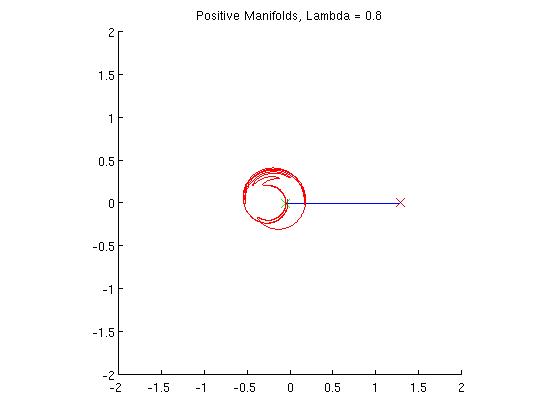
The red line is the unstable manifold and the blue is the stable. The point where they cross is a saddle point in the system and the other cross is the repelling point. I've only shown the positive manifolds (one side of the possible previous values) but the negative manifolds are just the reflection in the x-axis.
Sunday, 23 January 2011
Pwetty Pictures and a Presentation
So, this week when I thought about what to blog I left it pretty last minute. This means that instead of an (usually very interesting) insight into chaos I will share with you the presentation I gave on Friday for my project to students and lecturers. I have left the notes attached so you can follow what I spoke about as well.
One moment from someone else's presentation I would like to share is this:

Brilliant!!
The presentation itself was about business intelligence which does not really interest me but the image brought some light humour to the talk.
One moment from someone else's presentation I would like to share is this:

Brilliant!!
The presentation itself was about business intelligence which does not really interest me but the image brought some light humour to the talk.
Saturday, 15 January 2011
Nonlinearity gets all the fun
Nonlinearity is inherent in most systems before you make an assumption and reduce the beautiful complexity down to a boring bog standard linear system. There is a section in Strogatz that shows probably the most interesting thing you can do with linear systems (Chapter 5 section 3 page 138 onwards). And I only read it once because linear systems were dull and pretty repetitive long before A level.
Nonlinearity is pretty easy to understand. Take for example square numbers. You can make 4 by either multiplying 2 and 2 or -2 and -2. This means that, under the square operator, 4 has two (well, four really, but two are identical to the other two) possible previous values. This makes squaring a number nonlinear because tracking back you do not know whether two 2s or two -2s made the 4 you see at the moment. This particular brand of nonlinearity is called noninvertibility. You still following me?
Good. Right, to take this further we call the previous values of each number pre-images and the operation, a mapping. Now the quadratic (squaring) mapping that I am examining is:

what happens to z when a=2 and I vary lambda. This mapping does funny things depending on what I set lambda to. If it is between 0 and 1 then it behaves just like the squaring operator - each value of z has two pre-images as I iterate the map but in a circle radius=1-lambda around C the values have no pre-images. Now if I make lambda greater than 1, some values have two pre-images as before but the z values in the circle now have four pre-images.
Still with me? We can take this further but placing this property on curves not just points. A curve is just a line on a graph (an infinite set of points). Instead of looking backwards as we did with the points, we instead go forwards and see how the curve changes. It's first image is a circle, say. This curve then becomes the pre-image of the set of points of the circle under the mapping. And so on, forwards in time. It helps to look at the image below:
 You can see the curves collecting on (heading towards) one curve called a manifold (it's attracting). Now consider the relationship of the points and the curves. Because a curve is just a set of points. With noninvertibility inherent in the system, what happens it you take the manifold and reverse the mappings for all the points? Wild Chaos! Tracking the possible points and curves and how and why they interact is the next stage of my project - at least for certain ranges of values for C, a and lambda. This limitation is purely because my project has a time limit of a year.
I am currently working with a PhD student, Stefanie Hittmeyer (who incidentally produced the image above) who is working on the full problem in all its scope. She has been focused on the manifold part of it for the moment while I have been examining the fractal structure side. My work nicely compliments hers. This work is on the fore-front of chaos research. Now it may seem that all this has little value in the real world but the great thing about nonlinear and chaotic systems is that it can accurately mimic real world systems. This is a major advantage over linear systems because when taking a real world problem you have to reduce the picture you are looking at so you can describe it using the simplest tools. With this kind of research, no such reduction is necessary and you can understand the system in it's full complexity. So maybe it'll turn out that neurological signals in the brain will turn out to have similar properties to the mapping that I am examining and my research will contribute to a fuller understanding of how we came to have consciousness and help neurosurgeons get better at fixing the biochemical circuitry that makes us who we are. Or maybe, and more likely since this mapping is a reduction of the five dimensional Lorenz model, it will just help meteorologists get really, really good at predicting weather patterns.
Who knows? It's sort of like the laser - a solution created with no problem that has now become integral to our lifestyle. Just check out how many things it is used in! I hope you managed to follow all that to the end. If you have any specific questions please feel free to email me but I would much rather you follow that urge to take a deeper look yourself (even if that is just reading all the wiki pages). It's way more fun!
Nonlinearity is pretty easy to understand. Take for example square numbers. You can make 4 by either multiplying 2 and 2 or -2 and -2. This means that, under the square operator, 4 has two (well, four really, but two are identical to the other two) possible previous values. This makes squaring a number nonlinear because tracking back you do not know whether two 2s or two -2s made the 4 you see at the moment. This particular brand of nonlinearity is called noninvertibility. You still following me?
Good. Right, to take this further we call the previous values of each number pre-images and the operation, a mapping. Now the quadratic (squaring) mapping that I am examining is:

what happens to z when a=2 and I vary lambda. This mapping does funny things depending on what I set lambda to. If it is between 0 and 1 then it behaves just like the squaring operator - each value of z has two pre-images as I iterate the map but in a circle radius=1-lambda around C the values have no pre-images. Now if I make lambda greater than 1, some values have two pre-images as before but the z values in the circle now have four pre-images.
Still with me? We can take this further but placing this property on curves not just points. A curve is just a line on a graph (an infinite set of points). Instead of looking backwards as we did with the points, we instead go forwards and see how the curve changes. It's first image is a circle, say. This curve then becomes the pre-image of the set of points of the circle under the mapping. And so on, forwards in time. It helps to look at the image below:

I am currently working with a PhD student, Stefanie Hittmeyer (who incidentally produced the image above) who is working on the full problem in all its scope. She has been focused on the manifold part of it for the moment while I have been examining the fractal structure side. My work nicely compliments hers. This work is on the fore-front of chaos research. Now it may seem that all this has little value in the real world but the great thing about nonlinear and chaotic systems is that it can accurately mimic real world systems. This is a major advantage over linear systems because when taking a real world problem you have to reduce the picture you are looking at so you can describe it using the simplest tools. With this kind of research, no such reduction is necessary and you can understand the system in it's full complexity. So maybe it'll turn out that neurological signals in the brain will turn out to have similar properties to the mapping that I am examining and my research will contribute to a fuller understanding of how we came to have consciousness and help neurosurgeons get better at fixing the biochemical circuitry that makes us who we are. Or maybe, and more likely since this mapping is a reduction of the five dimensional Lorenz model, it will just help meteorologists get really, really good at predicting weather patterns.
Who knows? It's sort of like the laser - a solution created with no problem that has now become integral to our lifestyle. Just check out how many things it is used in! I hope you managed to follow all that to the end. If you have any specific questions please feel free to email me but I would much rather you follow that urge to take a deeper look yourself (even if that is just reading all the wiki pages). It's way more fun!
Saturday, 1 January 2011
Happy New Year!
This post I want to introduce my main project. The title is "Dynamics and Bifurcations of Two-Dimensional Noninvertible Maps". My plan for the project is available here to give you an idea of what I would like to achieve with it. Don't worry about all the scary words in it - the main idea is to find out what happens if I slightly permute the Mandelbrot set (a two dimensional map of Julia sets represented as a number set). Currently I'm focused on looking at how the Julia sets change. So far I have made lots of pretty pictures! as well as some observations on what happens.
Fractals are the most beautiful objects in chaos theory (wiki has a great introduction to them here). Simple definition is that fractals are shapes that are self-similar at all levels of magnitude - you cannot tell how zoomed in or out you are. The Mandelbrot is the most famous fractal and I love it because it is defined so simply but produces infinite complexity. My project considers the Mandelbrot as a single instance of a wider group of two-dimensional non-invertible maps. Noninvertible here means a many-to-one mapping forward in time i.e. if you back track there are many points that could have produced your original point.
Fractals were first observed in nature in the form of leaves on the trees. Ferns are made up of smaller ferns which are made up of even smaller ferns. The simplicity of defining a fractal has suggested that the information contained within the DNA of a plant to tell it what shape to grow into is in fact encoding fractal information. Another example would be one used recently in one of the Royal Institution Christmas Lectures - lungs. They translate a large volume of air onto a large surface area of blood vessels and they do it by being fractal. And recently there has been research that has found fractal patterns in semiconductor material at the quantum scale.
Fractals can be produced by nonlinear dynamics. This returns us back to the Lorenz equations and the butterfly attractor. The attractor found to describe the behaviour of the system is a fractal. Such a combination of parts of chaos theory is typical and continuing to find more links is very exciting. I have been finding bifurcation points and their stability in the fractal Julia sets as I permute the Mandelbrot set. Nonlinear dynamics can be produced by fractals. Thus my research is far reaching across the whole field of study. A field of study that is far reaching, interlinked and incredibly beautiful.
Fractals are the most beautiful objects in chaos theory (wiki has a great introduction to them here). Simple definition is that fractals are shapes that are self-similar at all levels of magnitude - you cannot tell how zoomed in or out you are. The Mandelbrot is the most famous fractal and I love it because it is defined so simply but produces infinite complexity. My project considers the Mandelbrot as a single instance of a wider group of two-dimensional non-invertible maps. Noninvertible here means a many-to-one mapping forward in time i.e. if you back track there are many points that could have produced your original point.
Fractals were first observed in nature in the form of leaves on the trees. Ferns are made up of smaller ferns which are made up of even smaller ferns. The simplicity of defining a fractal has suggested that the information contained within the DNA of a plant to tell it what shape to grow into is in fact encoding fractal information. Another example would be one used recently in one of the Royal Institution Christmas Lectures - lungs. They translate a large volume of air onto a large surface area of blood vessels and they do it by being fractal. And recently there has been research that has found fractal patterns in semiconductor material at the quantum scale.
Fractals can be produced by nonlinear dynamics. This returns us back to the Lorenz equations and the butterfly attractor. The attractor found to describe the behaviour of the system is a fractal. Such a combination of parts of chaos theory is typical and continuing to find more links is very exciting. I have been finding bifurcation points and their stability in the fractal Julia sets as I permute the Mandelbrot set. Nonlinear dynamics can be produced by fractals. Thus my research is far reaching across the whole field of study. A field of study that is far reaching, interlinked and incredibly beautiful.
Friday, 17 December 2010
Quantum Time Series
Currently I'm reading a book on quantum physics ("In Search of Schrodinger's Cat" by John Gribbon) and I was struck by the similar history of development it has with chaos theory i.e. no-one wants to admit it's really true and almost no-one really understands it. It has taken almost 100 years for quantum theory to be discovered, accepted and still it is only fully taught at university level after student have already been ingrained into thinking that electrons whoosh around the nucleus. I remember each level of school (middle school, pre-GCSE, GCSE) I took chemistry, I was told that everything I had been taught previously was wrong and too simple and here is the real thing! It got to the point that when I was choosing my A levels I did not pick Chemistry. I figured they would just lie to me again and I was better off learning the truth out of university textbooks. So I took Philosophy instead. I wonder whether others felt the same. I just wished they could have taught it correctly from the beginning and get over the fact that most 10-16 year-olds might not get it. Some will! Maybe in another hundred years quantum will be understood by enough people *cough* politicians *cough* that it can be taught straight from the beginning and not require almost a reprogramming of minds. Perhaps the same progress will happen for chaos theory. One can only hope.
This week my paper is on interaction of populations of competing species. Available here. It's quite a nice paper (longer than the last one). The purpose was to analyse how three equally competing species interact to change each other and their own population size over time. The time series plots provide examples of how systems require a certain amount of time to settle down to the final state. The equilibria that I talk about in the paper are fixed points for the system. They are the stable behaviour of the species interactions. So the species may start at different values (with the same parameters) but, over time, they will settle down to a fixed point (or periodic behaviour, or chaotic behaviour).
Taking the example of the pendulum again, when you set the pendulum in motion it will oscillate a few times and then settle back down to the lower central point. This is because it is damped by drag. This behaviour can be seen mathematically as a perturbation of initial conditions away from the stable equilibrium but over time it will return to that stable equilibrium, that stable position where it can hang without oscillating quite happily until the end of time. This stable equilibrium attracts all motion of the pendulum towards it so it is called an attracting fixed point.
Now opposite that stable equilibrium there is an unstable equilibrium. Right at the top of the circle that the pendulum could swing through. At this point the complete opposite happens to the point at the bottom. It repels all motion from it. A pendulum cannot hold itself up until the end of time (not with gravity anyway). So at the top we have a repelling fixed point and at the bottom we have an attracting fixed point. Mathematically the system makes sense.
Right, so now the easy bit is done, I'll add something a little harder to the end. You might be about to comment, "So what is happening when the pendulum in a clock oscillates on and on". So I'll tell you...
That is when the system has a period two oscillation if you set drag to zero (it is not exactly possible in the real world because drag does affect it due to not quite being zero which is why you had to keep winding them up). This means that when you set the motion going, you can get the pendulum to swing for the rest of time side to side. The distance and time period of the swing will be exactly the same for every oscillation. This is a stable period two oscillation and has a pretty sine or cosine curve on the time series plot.
Pendulum's can display chaotic motion. Just check this out. And each time you set it in motion it will swing and flip in a completely different way thanks to the effect of chaos - sensitive dependence on initial conditions!
This week my paper is on interaction of populations of competing species. Available here. It's quite a nice paper (longer than the last one). The purpose was to analyse how three equally competing species interact to change each other and their own population size over time. The time series plots provide examples of how systems require a certain amount of time to settle down to the final state. The equilibria that I talk about in the paper are fixed points for the system. They are the stable behaviour of the species interactions. So the species may start at different values (with the same parameters) but, over time, they will settle down to a fixed point (or periodic behaviour, or chaotic behaviour).
Taking the example of the pendulum again, when you set the pendulum in motion it will oscillate a few times and then settle back down to the lower central point. This is because it is damped by drag. This behaviour can be seen mathematically as a perturbation of initial conditions away from the stable equilibrium but over time it will return to that stable equilibrium, that stable position where it can hang without oscillating quite happily until the end of time. This stable equilibrium attracts all motion of the pendulum towards it so it is called an attracting fixed point.
Now opposite that stable equilibrium there is an unstable equilibrium. Right at the top of the circle that the pendulum could swing through. At this point the complete opposite happens to the point at the bottom. It repels all motion from it. A pendulum cannot hold itself up until the end of time (not with gravity anyway). So at the top we have a repelling fixed point and at the bottom we have an attracting fixed point. Mathematically the system makes sense.
Right, so now the easy bit is done, I'll add something a little harder to the end. You might be about to comment, "So what is happening when the pendulum in a clock oscillates on and on". So I'll tell you...
That is when the system has a period two oscillation if you set drag to zero (it is not exactly possible in the real world because drag does affect it due to not quite being zero which is why you had to keep winding them up). This means that when you set the motion going, you can get the pendulum to swing for the rest of time side to side. The distance and time period of the swing will be exactly the same for every oscillation. This is a stable period two oscillation and has a pretty sine or cosine curve on the time series plot.
Pendulum's can display chaotic motion. Just check this out. And each time you set it in motion it will swing and flip in a completely different way thanks to the effect of chaos - sensitive dependence on initial conditions!
Saturday, 4 December 2010
The Beginning...
Everyone starts somewhere.
I intend for this blog to be an aid for my Masters year. I intend to post papers I produce, thoughts on subjects I am taking, links to things that interest me (and maybe you) and perhaps the occasional insight into my thought processes. But as everyone knows, the best laid plans of mice and men...
I'm currently almost 'half' way through but I'll do my best to get you up to speed as best I can. My hope is to post once a week but don't hate me if I don't always manage it- I'll do my best to make up for it when possible.
So to give an overview...I am a final year student at the University of Bristol reading (as we say in the UK) Engineering Mathematics. We are currently 8 weeks into the year and so far I have written two papers, about to finish a third (this one is a group one) and none are getting published but they will all contribute to the degree I get out at the end. I have weekly labs, many hours of lectures and there is always work to be done in the form of my Final Year Project. Yep, I know, capitals seem silly here but the doom that surrounds it requires them really - it is, after all, contributing to 16.7% of my final degree classification which is more than my whole second year is worth. Oh, not forgetting the constant reading of required texts plus extensive reading around the subject in areas of interest.
As you can see, the workload is extensive and I bet you are wondering how I possibly have time to maintain this blog. Well, you see I hope that the small amount of extra work this may be will allow others to get a glimpse into an area of research that very few know about and even fewer really understand - Nonlinear Dynamics and Chaos - and how it fits in with engineering. Most people have heard of the Butterfly Effect but they do not really understand it - how exactly can a bat of the wings of a small butterfly change the weather on the other side of the world? Well, chaos theory explains phenomenon like this through understanding systems with "sensitive dependence on initial conditions".
Nonlinear dynamics and chaos is a rich field of research and crosses many other areas of science. I will not be spending this whole blog paraphrasing many better introductions and explanations. Instead, I will be discussing my studies directly and in each case will point the reader in the direction of preceding and/or related work. If nothing else, Wikipedia provides a great intro to the area. The best book for anyone of a mathematical persuasion is "Nonlinear Dynamics and Chaos" by Steven Strogatz. Any for those who are not, "Chaos" by James Gleick is a great read.
The relevance of this field to all science cannot be underestimated. Most engineers only look at systems in their most simplistic using assumptions that mean the system can be understood by classical mechanics. Those engineers trained in chaos can explore all the possibilities in the system. The best example of this is a system which most people have come across at some point: the pendulum. Remember the step the teachers did in class where they assumed that sin x = x for small angles and from then on the maths was really easy and you could understand how clocks work? Well, I know what happens when the pendulum swings over a big angle and it is really very elegant. Do you want to know too?
I intend for this blog to be an aid for my Masters year. I intend to post papers I produce, thoughts on subjects I am taking, links to things that interest me (and maybe you) and perhaps the occasional insight into my thought processes. But as everyone knows, the best laid plans of mice and men...
I'm currently almost 'half' way through but I'll do my best to get you up to speed as best I can. My hope is to post once a week but don't hate me if I don't always manage it- I'll do my best to make up for it when possible.
So to give an overview...I am a final year student at the University of Bristol reading (as we say in the UK) Engineering Mathematics. We are currently 8 weeks into the year and so far I have written two papers, about to finish a third (this one is a group one) and none are getting published but they will all contribute to the degree I get out at the end. I have weekly labs, many hours of lectures and there is always work to be done in the form of my Final Year Project. Yep, I know, capitals seem silly here but the doom that surrounds it requires them really - it is, after all, contributing to 16.7% of my final degree classification which is more than my whole second year is worth. Oh, not forgetting the constant reading of required texts plus extensive reading around the subject in areas of interest.
As you can see, the workload is extensive and I bet you are wondering how I possibly have time to maintain this blog. Well, you see I hope that the small amount of extra work this may be will allow others to get a glimpse into an area of research that very few know about and even fewer really understand - Nonlinear Dynamics and Chaos - and how it fits in with engineering. Most people have heard of the Butterfly Effect but they do not really understand it - how exactly can a bat of the wings of a small butterfly change the weather on the other side of the world? Well, chaos theory explains phenomenon like this through understanding systems with "sensitive dependence on initial conditions".
Nonlinear dynamics and chaos is a rich field of research and crosses many other areas of science. I will not be spending this whole blog paraphrasing many better introductions and explanations. Instead, I will be discussing my studies directly and in each case will point the reader in the direction of preceding and/or related work. If nothing else, Wikipedia provides a great intro to the area. The best book for anyone of a mathematical persuasion is "Nonlinear Dynamics and Chaos" by Steven Strogatz. Any for those who are not, "Chaos" by James Gleick is a great read.
The relevance of this field to all science cannot be underestimated. Most engineers only look at systems in their most simplistic using assumptions that mean the system can be understood by classical mechanics. Those engineers trained in chaos can explore all the possibilities in the system. The best example of this is a system which most people have come across at some point: the pendulum. Remember the step the teachers did in class where they assumed that sin x = x for small angles and from then on the maths was really easy and you could understand how clocks work? Well, I know what happens when the pendulum swings over a big angle and it is really very elegant. Do you want to know too?
Subscribe to:
Posts (Atom)